ASSO 대비
| source | |
| type | 📌 개발노트 |
| topics | 100-데이터분석 & AI 101 머신러닝 |
| index | 자격증 |
| tags |
!pip install seaborn
인덱스,시리즈,데이터프레임
loc,iloc
apply
DataFrame 데이터 접근 방법
보통 axis 가 0이면 가로 , 1일면 세로임
기본 함수들 : https://ordo.tistory.com/37
import pandas as pd
import numpy as np
import matplotlib.pyplot as plt
import seaborn as sns
1. 데이터 불러오기 및 구성 확인
기본
import pandas as pd

# <span id="불러오기"></span>불러오기
df = pd.read_csv("경로")
"""
index_col=0**: 첫 번째 컬럼을 인덱스로 사용
index_col='컬럼이름'**: 해당 컬럼을 인덱스로 사용
"""

# <span id="확인-상하위-5개"></span>확인 상하위 5개
df.head()
df.tail()

# <span id="데이터프레임-정보출력"></span>데이터프레임 정보출력
df.info() # 컬럼, not-null 개수, dtype

# <span id="각컬럼의-통계-요약-count는-결측치가-아닌-것의-개수"></span>각컬럼의 통계 요약, count는 결측치가 아닌 것의 개수
# <span id="일반적으론-수치형만"></span>일반적으론 수치형만
df.describe() # count, mean, std, min, 25%, 50%, 75%, max
# <span id="범주형object"></span>범주형(object)
df.describe(include="O")
# <span id="count-값의-개수결측치-제외"></span>count: 값의 개수(결측치 제외)
#unique: 고유값 개수
#top: 가장 많이 나온 값(최빈값)
#freq: 최빈값의 빈도수


# <span id="행을-식별하는-라벨-보통-인덱스라고-부름"></span>행을 식별하는 라벨 ( 보통 인덱스라고 부름)
# <span id="행의-길이와-같음-기본적으론-rangeindex가-부여"></span>행의 길이와 같음, 기본적으론 rangeindex가 부여
df.index

# <span id="열을-식별하는-라벨"></span>열을 식별하는 라벨

# <span id="각-열에-어떤-값이-있는지"></span>각 열에 어떤 값이 있는지
df[].values # 데이터프레임에서도 사용가능
df[].unique() #데이터프레임에서는 사용불가

# <span id="df-에서-각-열의-타입"></span>df 에서 각 열의 타입
df.dtypes
# <span id="시리즈에서의-타입-"></span>시리즈에서의 타입
df.dtype

# <span id="행열-개수-반환"></span>행열 개수 반환
df.shape # 결과 : (행,열)

# <span id="행열-바꾸기-"></span>행열 바꾸기
df.T

# <span id="정렬"></span>정렬
s_sorted = s.sort_index() # 인덱스 기준 정렬
s_sorted = s.sort_values() # 값 기준 정렬
시각화
https://diane-space.tistory.com/128
시본시각화
import matplotlib.pyplot as plt
# <span id="원형차트로-벨류의-비율을-보여주고픔"></span>원형차트로 벨류의 비율을 보여주고픔
plt.figure(figsize = (8, 5))
df['voc_trt_perd_itg_cd'].value_counts().plot(kind = 'pie', autopct = '%.2f%%')
plt.show()

# <span id="특정-컬럼의-값의-데이터를-10개의-구간으로-나눠-히스토그램으로"></span>특정 컬럼의 값의 데이터를 10개의 구간으로 나눠 히스토그램으로
plt.hist(wine['alcohol'], bins=10)

# <span id="산점도"></span>산점도
# <span id="아래-둘다-같음"></span>아래 둘다 같음
wine.plot.scatter(x='rat_ca', y='quality')
plt.scatter(wine['rat_ca'], wine['quality'])

# <span id="선그래프"></span>선그래프
plt.plot(range(1, 51), accs) # 순서대로 x, y 값
# <span id="여러-옵션들"></span>여러 옵션들
plt.title('Accuracy')
plt.xlabel('epochs')
plt.ylabel('accuracy')
plt.legend()
plt.grid(True)

# <span id="막대그래프-"></span>막대그래프
df.plot.bar()
# <span id="박스플롯-"></span>박스플롯
df.plot.box()

# <span id="시본-버전"></span>시본 버전
import seaborn as sns
# <span id="산점도"></span>산점도
tips = sns.load_dataset("tips")
sns.scatterplot(x="total_bill", y="tip", data=tips)

# <span id="막대그래프"></span>막대그래프
sns.barplot(x="day", y="total_bill", data=tips)

# <span id="히스토그램"></span>히스토그램
sns.histplot(x="total_bill", data=tips, bins=20, kde=True)

# <span id="페어플롯-여러-변수-간-관계-시각화"></span>페어플롯 (여러 변수 간 관계 시각화)
iris = sns.load_dataset("iris")
sns.pairplot(data=iris, hue="species")
| 함수 | 주요 용도 | 대표 시각화 |
|---|---|---|
| kdeplot | 연속형 데이터 분포 | 밀도곡선 |
| pairplot | 다변량 변수간 관계, 분포 | 산점도/히스토그램 |
| countplot | 범주형 데이터 빈도 | 막대그래프 |
| heatmap | 2D 데이터의 값 크기/패턴 | 색상 행렬 |
| boxplot | 수치형 데이터 분포/이상치 | 상자수염그림 |
2. 데이터 정제
1) 결측치 확인
# <span id="각-컬럼별-결측치가-몇개-존재하는지-"></span>각 컬럼별 결측치가 몇개 존재하는지
df.isnull().sum()
df.isna().sum() # 이두개 완전히같음
# <span id="notna나-notnull의-경우-결측값이면-false를-반환합니다"></span>`notna`나 `notnull`의 경우 결측값이면 `False`를 반환합니다.

# <span id="특정값이-몇개-존재하는-지-"></span>특정값이 몇개 존재하는 지
(df['column명'] == '특정').sum()
df2=df1.replace('_',None)

# <span id="특정열-value의-개수를-확인"></span>특정열 value의 개수를 확인
# <span id="시리즈를-반환"></span>시리즈를 반환
df["열이름"].value_counts()

# <span id="특정열-드록"></span>특정열 드록
df5=df5.drop(columns=['new_date','opn_nfl_chg_date','cont_fns_pam_date'])
value_counts 옵션들
https://zzinnam.tistory.com/entry/pandas-valuecounts-%ED%95%A8%EC%88%98
| 옵션 | 설명 | 기본값 |
|---|---|---|
| normalize | 비율로 반환할지 여부 | False |
| sort | 결과를 정렬할지 여부 | True |
| ascending | 오름차순 정렬 여부 | False |
| dropna | 결측치(NaN)를 제외할지 여부 | True |
2) 결측치 처리
결측치 제거
50퍼가넘는건 제거
# <span id="결측치가-50-이상인-컬럼을-드롭-"></span>결측치가 50% 이상인 컬럼을 드롭
threshold = len(df) * 0.5
df_cleaned = df.loc[:, df.isnull().sum() < threshold]
# <span id="같은의미의-코드들-thresh-결측치가-몇개-이상이면-드롭"></span>같은의미의 코드들 thresh 결측치가 몇개 이상이면 드롭
# <span id="subset-dropna메서드를-수행할-레이블을-지정합니다"></span>`subset` : `dropna`메서드를 수행할 레이블을 지정합니다.
df.dropna(axis=1, thresh=int(len(df)*0.5)+1)
df.loc[:, df.isnull().mean() < 0.5]

# <span id="dropna-axis-기본-0-행"></span>dropna axis 기본 0 (행)
df.dropna() # 결측치잇는 행제거
# <span id="결측치-있는-특정컬럼-행제거"></span>결측치 있는 특정컬럼 행제거
df = train.dropna(subset=['country','workclass'])
결측치 replace
# <span id="결측치를-중앙값으로-변환"></span>결측치를 중앙값으로 변환
df4 = df3.fillna({'age_itg_cd':df3['age_itg_cd'].median()})
# <span id="최빈값으로"></span>최빈값으로
df5=df5.fillna({'cust_dtl_ctg_itg_cd':df5['cust_dtl_ctg_itg_cd'].mode()[0]})
3) 데이터 형변환
astype:
모든 값이 지정한 타입으로 변환 가능해야 하며, 불가능하면 에러가 납니다.to_numeric:
변환 불가능한 값이 있어도 옵션(errors='coerce')을 주면 NaN으로 처리해 더 유연하게 작동합니다
# <span id="astype"></span>astype
df4['age_itg_cd']=df4['age_itg_cd'].astype(int)

# <span id="시리즈"></span>시리즈
pd.to_numeric(s, errors='coerce')
# <span id="데이터프레임"></span>데이터프레임
df_numeric = df.apply(pd.to_numeric, errors='coerce')
4) 특정 데이터타입 선택
# <span id="예-object문자열-타입-컬럼만-선택"></span>예: object(문자열) 타입 컬럼만 선택
object_cols = df.select_dtypes(include=['object']).columns
# <span id="예-object-타입-컬럼을-float으로-변환"></span>예: object 타입 컬럼을 float으로 변환
df[object_cols] = df[object_cols].astype('float')
# <span id="특정타입의-컬럼을-선택해서-이렇게-형변환도-가능"></span>특정타입의 컬럼을 선택해서 이렇게 형변환도 가능
5) 분류 인코딩
분류를 인코딩하는데는 라벨인코딩과 원핫인코딩이있음
라벨은 value가 a,b,c,d 이러면 이걸걍 숫자로 단순 변환
원핫은 value가 a,b,c,d 이러면 컬럼_a이렇게 새로 컬럼을 만듬
원핫은 값이 0 아니면 1임ㅋㅋ
| 구분 | 라벨 인코딩 | 원핫 인코딩 |
|---|---|---|
| 변환 방식 | 각 범주를 정수로 매핑 | 각 범주를 별도 열로 만들고 0/1로 표시 |
| 사용 상황 | 순서 없는 범주, 트리 계열 모델, 목표변수 | 순서 없는 범주, 대부분의 모델, 입력 변수 |
| 장점 | 간단, 변수 수 증가 없음 | 순서/크기 정보 왜곡 없음, 대부분 모델에 안전 |
| 단점 | 숫자 간 순서 오해 가능 | 변수(열) 수 증가, 희소 행렬 |
# <span id="안보고-한번에-오브젝트-확인하려면-아래방법쓰면됨"></span>안보고 한번에 오브젝트 확인하려면 아래방법쓰면됨
cols = train.select_dtypes(include='object').columns cols = train.columns[train.dtypes == object]

# <span id="라벨-인코딩"></span>라벨 인코딩
from sklearn.preprocessing import LabelEncoder
le = LabelEncoder()
df5['cust_clas_itg_cd'] = le.fit_transform(df5['cust_clas_itg_cd'])
# <span id="만약-분리후에햇고-위의-인코딩방식이랑-같게-인코딩하려면"></span>만약 분리후에햇고 위의 인코딩방식이랑 같게 인코딩하려면
le.transform(test[col])
# <span id="r-g-b-가-가각-012-로-라벨인코딩되엇을때-"></span>R, g, b 가 가각 0,1,2 로 라벨인코딩되엇을때
# <span id="transform은-그기준에-맞춰서-라벨인코딩해줌"></span>transform은 그기준에 맞춰서 라벨인코딩해줌
# <span id="traintest-분리-전에-fit_transform을-하면-안-되는-이유"></span>train/test 분리 전에 fit_transform을 하면 안 되는 이유
# <span id="test-데이터의-정보를-미리-알고-학습하는-것과-같음"></span>test 데이터의 정보를 미리 알고 학습하는 것과 같음

# <span id="원핫인코딩-판다스의-함수임"></span>원핫인코딩 , 판다스의 함수임
df6=pd.get_dummies(df5,columns = cat_cols.drop('cust_clas_itg_cd'))
3. 데이터 변환
test,val,train데이터 분할
- train(학습 데이터): 모델을 학습시키는 데 사용
- validation(검증 데이터): 하이퍼파라미터 튜닝, 모델 선택 등에 사용 (학습에는 사용하지 않음)
- test(테스트 데이터): 최종적으로 모델의 성능을 평가하는 데 사용 (학습과 검증에 모두 사용하지 않음)
from sklearn.model_selection import train_test_split
# <span id="xy-분할"></span>x,y 분할
X = df6.drop(target, axis=1) # axis 기본row 삭제
y = df6[target]
# <span id="아래처럼-처리도-가능-단-원본이-수정됨"></span>아래처럼 처리도 가능 단 원본이 수정됨
y = train.pop("income")
x = train
# <span id="traintest-분리"></span>train,test 분리
# <span id="stratify-비율-유지"></span>stratify : 비율 유지
X_train, X_test, y_train, y_test = train_test_split(X, y, test_size=0.2, stratify=y, random_state=42)
# <span id="traintest-분리"></span>train,test 분리
X_train, X_valid, y_train, y_valid = train_test_split(X_train, y_train, test_size=0.2, random_state=2021, stratify=y_train)
스케일링
표준화(정규분포화)
from sklearn.preprocessing import StandardScaler
scaler = StandardScaler()
X_train = scaler.fit_transform(X_train) # 평균0 표편 1
# <span id="fit하지않음"></span>fit하지않음
X_test = scaler.transform(X_test) # 이건 X_train에서 계산 한 평균,표편을 사용해서 표준화
정규화
from sklearn.preprocessing import MinMaxScaler
scaler = MinMaxScaler()
df_normalized = scaler.fit_transform(df)
로버트: 중앙값과 사분위값활용, 이산치영향최소화
from sklearn.preprocessing import RobustScaler
scaler = RobustScaler()
train[col] = scaler.fit_transform(train[col])
test[col] = scaler.transform(test[col])
4. 학습
일반 머신러닝
분류
# <span id="로지스틱"></span>로지스틱
from sklearn.linear_model import LogisticRegression
lr_model = LogisticRegression(C=10, max_iter = 2000)
lr_model.fit(X_train, y_train)

# <span id="knn"></span>knn
from sklearn.neighbors import KNeighborsClassifier
model = KNeighborsClassifier(n_neighbors=)

# <span id="결정트리"></span>결정트리
from sklearn.tree import DecisionTreeClassifier
model = DecisionTreeClassifier(max_depth=, random_state=)

# <span id="랜덤포레스트"></span>랜덤포레스트
from sklearn.ensemble import RandomForestClassifier
model = RandomForestClassifier(n_estimators=, random_state=)

# <span id="xgboost-트리이용"></span>xgboost 트리이용
from xgboost import XGBClassifier
model = XGBClassifier(n_estimators= )

# <span id="lightgbm-트리이용"></span>lightgbm 트리이용
from lightgbm import LGBMClassifier
model = LGBMClassifier(n_estimators=)
회귀
from sklearn.linear_model import LinearRegression
model = LinearRegression(  )

from sklearn.neighbors import KNeighborsRegressor
moedel = KNeighborsRegressor(n_neighbors=)

from sklearn.tree import DecisionTreeRegressor
model = DecisionTreeRegressor()

from sklearn.ensemble import RandomForestRegressor
model = RandomForestRegressor()

from xgboost import XGBRegressor
model = XGBRegressor( )

from lightgbm import LGBMRegressor
model = LGBMRegressor()
딥러닝
회귀는 출력레이가 하나 분류는 출력레이어가 두개
개념
- Activation Function (활성화 함수)
- 역할: 뉴런의 출력에 비선형성을 추가해 복잡한 패턴 학습 가능.
- 주요 함수:
relu: 은닉층에서 주로 사용 (음수는 0, 양수는 그대로).sigmoid: 이진 분류의 출력층에서 사용 (0~1 확률 출력).softmax: 다중 분류의 출력층에서 사용 (클래스별 확률 합 1).linear: 회귀 문제의 출력층에서 사용 (연속값 예측).
- 분류 vs 회귀:
- 분류: 출력층에
sigmoid(이진),softmax(다중). - 회귀: 출력층에 활성화 함수 없음.
- 분류: 출력층에
- Optimizer (최적화 알고리즘)
- 역할: 손실 함수를 최소화하는 가중치 업데이트 방향 결정.
- 주요 옵티마이저:
adam: Adaptive Moment Estimation (기본 추천).sgd: Stochastic Gradient Descent (학습률 조절 필요).rmsprop: RNN에 적합.
- 분류 vs 회귀: 문제 유형과 무관하게 동일하게 사용 가능.
- Loss Function (손실 함수)
- 역할: 예측값과 실제값의 오차를 계산.
- 주요 손실 함수:
- 분류:
binary_crossentropy: 이진 분류 (출력층sigmoid와 함께 사용).categorical_crossentropy: 다중 분류 (출력층softmax와 함께 사용).sparse_categorical_crossentropy:다중분류- 원핫인코딩안됏으면 이거사용
- 회귀:
mse(Mean Squared Error): 연속값 예측.mae(Mean Absolute Error): 이상치에 덜 민감.
- 분류:
- 분류 vs 회귀:
- 분류: 크로스 엔트로피 계열 사용.
- 회귀: MSE/MAE 사용.
- EarlyStopping
- 역할: 검증 데이터의 손실(val_loss)이 개선되지 않을 때 학습을 조기 중단.
- 주요 파라미터:
monitor: 모니터링할 지표 (예:val_loss).patience: 개선이 없을 때 몇 epoch까지 기다릴지 (예: 4).mode: 최소화(min) 또는 최대화(max) 방향 설정.
- ModelCheckpoint
- 역할: 모델의 가중치를 파일로 저장 (예:
best_model.keras). - 주요 파라미터:
monitor: 저장 기준 지표 (예:val_loss).save_best_only: 가장 좋은 모델만 저장.verbose: 저장 시 로그 출력.
- 역할: 모델의 가중치를 파일로 저장 (예:
신경망에서의원핫인코딩 > to_categorical
from keras.utils import to_categorical
y_train_ohe = to_categorical(y_train)
y_test_ohe = to_categorical(y_test)
| 구분 | to_categorical | pd.get_dummies |
|---|---|---|
| 주 용도 | 정답 레이블(타깃) 인코딩 | 입력 데이터(피처) 인코딩 |
| 입력 | 1차원 정수 배열 | 시리즈/데이터프레임(범주형) |
| 출력 | 넘파이 배열(2D) | 판다스 데이터프레임 |
| 대상 | 보통 y(정답) | 보통 X(입력 피처) |
| 다중 컬럼 지원 | X | O |
| 문자열 지원 | X (정수만) | O |
| 사용 예시 | 딥러닝 분류 레이블 | 머신러닝 피처 전처리 |
구현
- 첫번째 Hidden Layer : unit 64 , activation='relu'
- 두번째 Hidden Layer : unit 32 , activation='relu'
- 세번째 Hidden Layer : unit 16 , activation='relu'
- 각 Hidden Layer 마다 Dropout 0.2 비율로 되도록 하세요.
- EarlyStopping 콜백을 적용하고 ModelCheckpoint 콜백으로 validation performance가 좋은 모델을 best_model.keras 모델로 저장하세요.
- batch_size는 10, epochs는 10으로 설정하세요.
import tensorflow as tf
from tensorflow import keras
from tensorflow.keras.models import Sequentia, load_model
from tensorflow.keras.layers import Dense, Dropout
from tensorflow.keras.callbacks import EarlyStopping, ModelCheckpoint

model = Sequential([
    Dense(64,activation='relu',input_shape=(X_train.shape[1],)),# 입력층
    Dropout(0.2),
    Dense(32,activation='relu')
    Dropout(0.2),
    Dense(16,activation='relu')
    Dropout(0.2),
    Dense(32,activation='sigmoid')# 출력층
    # 출력시 분류면 featurer개수, 회귀면 1
    # activation 함수는 분류(이중:sigmoid,다중:softmax) 회귀면없어도됨

])

model.compile(
    optimizer = 'adam',
    loss = 'binary_crossentropy',
    # 분류 categorical_crossentropy binary_crossentropy
    # 분륜데 원핫 레이블 되지 않았으면 : sparse_categorical_crossentropy
    # 회귀 : mse or mae
    metrics = ['acc']  # 평가지표로 acc(정확도르 사용할것임)
    # 분류 'acc', 'AUC'
    # 보통 회귀 : 'mae', 'mse'
)
es = EarlyStopping(monitor='val_loss', patience=4, mode='min', verbose=1)

mc = ModelCheckpoint('best_model.keras', monitor='val_loss', save_best_only=True, verbose=1)

history = model.fit(X_train, y_train,
    batch_size=10,
    epochs=10,
    callbacks=[es, mc],
    validation_data=(X_test, y_test),
    verbose=1)

# <span id="ohe는-원핫인코딩한데이터"></span>ohe는 원핫인코딩한데이터
history = model.fit(X_train, y_train_ohe, batch_size=10, epochs=10, callbacks=[es,mc], validation_data=(X_test, y_test_ohe), verbose=1)

# <span id="구녕조정"></span>구녕조정
model.save('voc_model.keras')
5. 결과 확인및 시각화
분류
값 예측 잘하나확인
원핫인코딩 되었을땐 각클래스에 맞는 확률을 리턴하기에 argmax를이용해야함
가장 높게 예측한걸 예측한클래스로 생각한다는 말임
from sklearn.metrics import confusion_matrix, classification_report
import seaborn as sns

y_lr_predict = lr_model.predict(X_test)
cm = confusion_matrix(y_test,y_lr_predict)
sns.heatmap(
    cm,
    annot =True # 각 셀에 값 표시
    fmt = 'd', # 정수형으로 표시
    cmap = 'Blues' # 색상
)
plt.xlabel('Predicted')
plt.ylabel('Actual')

classification_report(y_test, y_lr_predict)

## <span id="원핫인코딩되어서"></span>원핫인코딩되어서
y_test_pred = model.predict(X_test, batch_size=10, verbose=1)
y_test = np.argmax(y_test_ohe, axis=1)
y_test_pred = np.argmax(y_test_pred, axis=1)

from sklearn.metrics import accuracy_score
accuracy_score(y_test, y_test_pred)
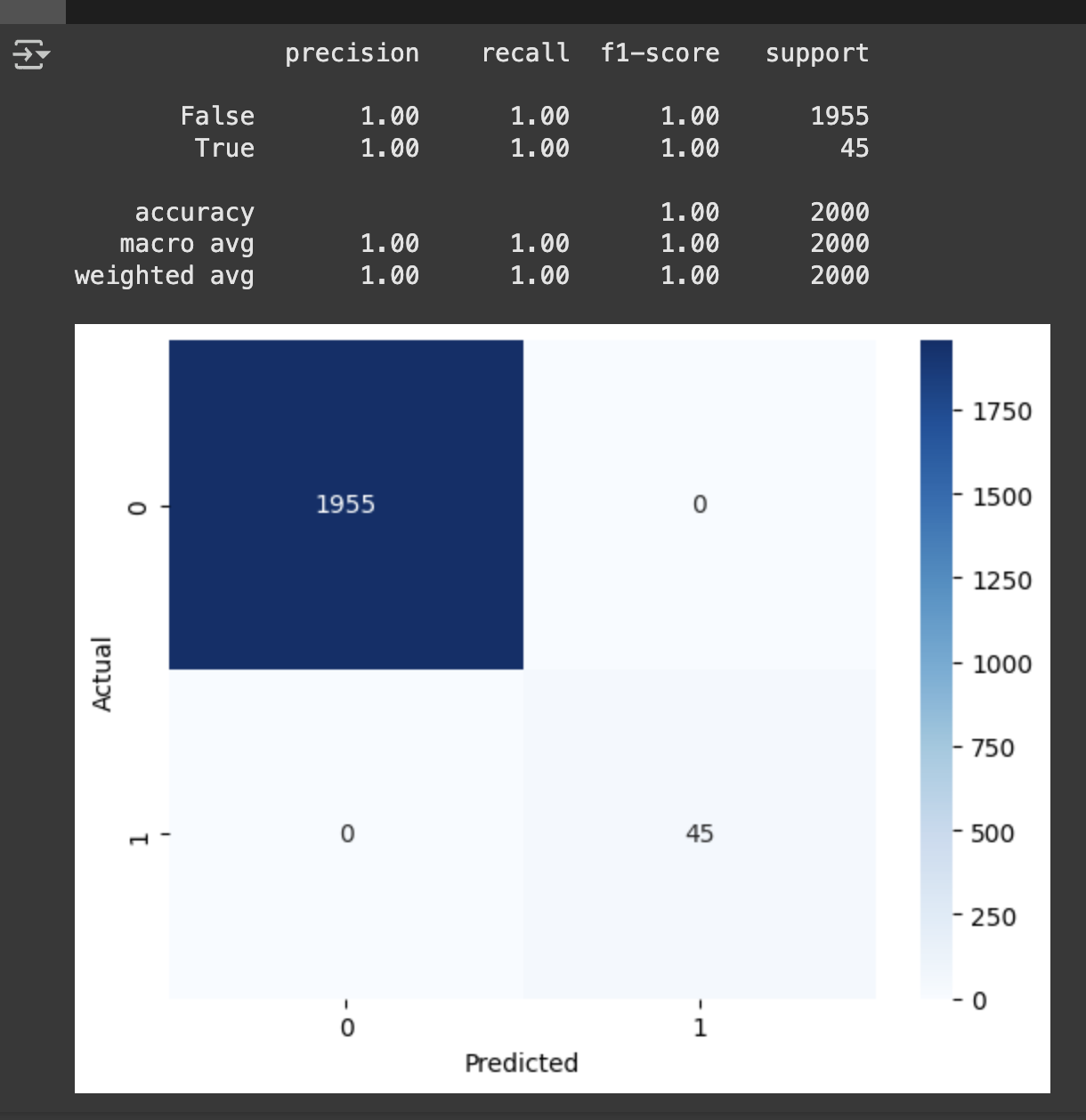
- macro avg : 각 클래스의 정밀도, 재현율, F1-score의 단순 평균(여기선 모두 1.00).
- weighted avg: 각 클래스의 support(데이터 개수)로 가중평균(여기선 모두 1.00).
loss 확인 - history이용함
plt.figure(figsize=(10,5))
plt.plot(history.history['acc'])
plt.plot(history.history['val_acc'])
plt.title('Model Accuracy')
plt.xlabel('Epochs')
plt.ylabel('Accuracy')
plt.legend(['Train','Validation'], loc='lower right')

plt.figure(figsize=(10,5))
plt.plot(history.history['loss'], 'b', label='Train Loss')
plt.plot(history.history['val_loss'], 'y', label='validaton Loss')
plt.xlabel('Epochs')
plt.ylabel('Loss')
plt.legend()
딥러닝
회귀
from sklearn.metrics import mean_squared_error, mean_absolute_error,r2_score

y_pred = model.predict(x_test)

#결과
print(mean_squared_error(y_test, y_pred, squared=False)) # RMSE를 반환
print(mean_absolute_error(y_test, y_pred))
print(r2_score(y_test, y_pred))


# <span id="회귀계수-가중치-확인-"></span>회귀계수 = 가중치 확인 :
model.coef_

# <span id="편향y절편-"></span>편향(y절편) =
model.intercept_